
ニューラルネットワーク
| 機械学習および データマイニング |
|---|
 |
|
|
︵人工知能の分野で︶ニューラルネットワーク︵英: neural network; NN、神経網︶は、生物の学習メカニズムを模倣した機械学習手法として広く知られているものであり[1]、﹁ニューロン﹂と呼ばれる計算ユニットをもち、生物の神経系のメカニズムを模倣しているものである[1]。人間の脳の神経網を模した数理モデル[2]。模倣対象となった生物のニューラルネットワーク︵神経網︶とはっきり区別する場合は、人工ニューラルネットワーク (英: artificial neural network) と呼ばれる。
以下では説明の都合上[注釈 1]、人工的なニューラルネットワークのほうは﹁人工ニューラルネットワーク﹂あるいは単に﹁ニューラルネットワーク﹂と呼び、生物のそれは﹁生物のニューラルネットワーク﹂あるいは﹁生物の神経網﹂、ヒトの頭脳のそれは﹁ヒトのニューラルネットワーク﹂あるいは﹁ヒトの神経網﹂と表記することにする。

生物のニューロン
人工ニューラルネットワークを理解するには、そもそもそれがどのようなものを模倣しようとしているの知っておく必要があるので説明する。ヒトの神経系にはニューロンという細胞があり、ニューロン同士は互いに軸索 (axon) と樹状突起 (dendrite) を介して繋がっている。ニューロンは樹状突起で他の神経細胞から情報を受け取り、細胞内で情報処理してから、軸索で他のニューロンに情報を伝達する[3]。そして、軸索と樹状突起が結合する部分をシナプス(synapse)という[3][1]︵右図も参照。クリックして拡大して見ていただきたい。紫色の部分がひとつのニューロンであり、Dendrite, Axonなどが示されている。︶。 このシナプスの結合強度というのは、外的な刺激に反応してちょくちょく変化する。このシナプス結合強度の変化こそが生物における﹁学習﹂のメカニズムである[1]。[注釈 2]

人工ニューロン
ヒトの神経網を模した人工ニューラルネットワークでは、計算ユニットが︽重み︾を介して繋がり、この︽重み︾がヒトの神経網のシナプス結合の﹁強度﹂と似た役割を担っている[1]。各ユニットへの入力は︽重み︾によって強さが変化するように作られており、ユニットにおける関数計算に影響を与える。ニューラルネットワークというのは、入力用ニューロンから出力用ニューロンへと向かって計算値を伝播させてゆくが、その過程で︽重み︾をパラメータとして利用し、入力の関
数を計算する。︵ただし計算値が出力用ニューロンへと伝播されてゆくというだけでは入力パターンからある決まった出力パターンが出るだけなので、さほど有益というわけではない[4]。︶︽重み︾が変化することで﹁学習﹂が起きる[1]︵ここが重要なのである[4]︶。
︵右図も参照のこと。右図で﹁weights﹂や、丸で囲まれた﹁w﹂が縦に並んでいるのが︽重み︾である。︶
生物のニューラルネットワークに与えられる外的刺激に相当するものとして、人工ニューラルネットワークでは﹁訓練データ﹂が与えられる[1]。いくつか方法があるが、たとえば訓練データとして入力データと出力ラベルが与えられ、たとえば何かの画像データとそれについての正しいラベルが与えられる︵たとえばリンゴの画像データとappleというラベル、オレンジの画像データとorangeというラベルが与えられる︶。ある入力に対して予測される出力が本当のラベルとどの程度一致するかを計算することで、ニューラルネットワークの︽重み︾についてフィードバックを得られ[1]、ニューロン間の︽重み︾は誤差︵予測誤差︶に応じて、誤差が減少するように調整される[1]。多数のニューロン間で︽重み︾の調整を繰り返し行うことで次第に計算関数が改善され、より正確な予測をできるようになる。︵たとえばオレンジの画像データを提示されると﹁orange﹂と正しいラベルを答えられるようになる[1]。︶
︽重み︾の調整方法の代表的なものがバックプロパゲーションである[4]。
なお、ヒトのニューロンを模したユニットは人工ニューロンあるいはノードと呼ばれる。

相互作用ニューラルネットワークモデルの一例
右図の、多数のユニットが結合しネットワークを構成している数理モデルは、ニューラルネットワークのほんの一例である。︵実際にはニューロンの数もさまざまに設定可能であるし、結合のしかたもさまざまに設定可能である。右図はあくまで、とりあえず説明にとりかかるための﹃一例﹄と理解いただきたい。
ユニットの構成︵例: 線形変換の次元、非線形変換の有無・種類︶やネットワークの構造︵例: ユニットの数・階層構造・相互結合、入出力の再帰︶に関して様々な選択肢があり、様々なモデルが提唱されている。︶
各ユニットは入力の線形変換を必ず含み、多くの場合それに後続する非線形変換を含む︵ ︶。
︶。
ニューラルネットワークは機械学習のモデルとして利用され、分類・回帰・生成など様々なクラスのタスクに教師あり/教師なし問わず利用される。利用分野にはパターン認識やデータマイニング︵例: 画像認識、レコメンデーション︶が挙げられる。学習法は誤差逆伝播法が主流である。 三層以上のニューラルネットワークは可微分で連続な任意関数を近似できることが証明されている︵線形分離不可能な問題を解ける︶。 形式ニューロンなど研究の源流としては生物の神経系の探求であるが、その当初から、それが実際に生物の神経系のシミュレーションであるか否かについては議論がある[注釈 3]。生物学と相互の進展により、相違点なども研究されている。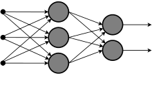
多層パーセプトロンの模式図

畳み込みニューラルネットワーク
概要[編集]


 ︶。
︶。
ニューラルネットワークは機械学習のモデルとして利用され、分類・回帰・生成など様々なクラスのタスクに教師あり/教師なし問わず利用される。利用分野にはパターン認識やデータマイニング︵例: 画像認識、レコメンデーション︶が挙げられる。学習法は誤差逆伝播法が主流である。 三層以上のニューラルネットワークは可微分で連続な任意関数を近似できることが証明されている︵線形分離不可能な問題を解ける︶。 形式ニューロンなど研究の源流としては生物の神経系の探求であるが、その当初から、それが実際に生物の神経系のシミュレーションであるか否かについては議論がある[注釈 3]。生物学と相互の進展により、相違点なども研究されている。
歴史[編集]
第二次世界大戦の最中の1943年のこと、ウォーレン・マカロックとウォルター・ピッツが神経回路網理論を提出したが︵形式ニューロンを参照︶、この理論は現実の脳と比べてあまりに単純化するものだったので当時はほとんど注目されなかった。また1949年にドナルド・ヘッブが神経回路の学習理論として発表した ﹁シナプスの可塑性の理論﹂ も " 単なる机上の空論 " の扱いを受けてしまった[5]。 状況が変わりはじめたのは1967年のことで、同年に小脳の神経回路網の構造が明らかになり[6]、そのおかげで上述のマカロック、ピッツ、ヘッブらの理論が現実の小脳をうまくモデル化していることが分かり、すでに発表されて10年ほど経っていたパーセプトロンが俄然ブームとなった[5]。 ところが1970年代になるとマービン・ミンスキーとシーモア・パパートがパーセプトロンの限界を数学的に証明したことで、神経回路網的手法に対する期待が一気にしぼみ、その研究者の数が急激に減ってしまった[5]。それでも地道な研究を続けていた人はおり[5]、︵1986年にデビッド・ラメルハートらがバックプロパゲーション︵誤差 逆伝播法︶を再発見︵再提案︶したことで、それまでの限界を突破する道がとうとう開け︶ ﹁ニューラルネットワーク﹂として多くの研究者の注目を浴びるようになった[5]。年表[編集]
●1943年、ウォーレン・マカロックとウォルター・ピッツが形式ニューロンを発表した。 ●1958年、フランク・ローゼンブラットがパーセプトロンを発表した。 ●1969年、マービン・ミンスキーとシーモア・パパートが著書﹃パーセプトロン﹄の中で、単純パーセプトロンは線形分離不可能なパターンを識別できない事を示した。 ●1979年、福島邦彦がネオコグニトロンを発表し、文字認識に使用し、後にこれが畳み込みニューラルネットワークへと発展する。 ●1982年、ジョン・ホップフィールドによってホップフィールド・ネットワーク︵再帰型ニューラルネットワーク︶が提案された。 ●1985年、ジェフリー・ヒントンらによりボルツマンマシンが提案された。 ●1986年、デビッド・ラメルハートらにより誤差逆伝播法︵バックプロパゲーション︶が提案︵再発見︶された。 ●1988年、畳み込みニューラルネットワークを本間俊光らが音素の認識に[7]、1989年にヤン・ルカンらが文字の認識に使用した[8][9]。LeCunらの多層の畳み込みニューラルネットワークは後にディープラーニングの一種に分類されることになる。 ●2006年、ジェフリー・ヒントンらによりオートエンコーダ[10]およびディープ・ビリーフ・ネットワーク[11]が提案され、この理論が、2010年代にディープラーニングと呼ばれる分野を形成した。代表的な人工ニューラルネットワーク[編集]
順伝播型ニューラルネットワーク[編集]
順伝播型ニューラルネットワーク︵フィードフォワードニューラルネットワーク、英: Feed-forward Neural Network; FFN, FFNN︶は内部に循環を持たないニューラルネットワークの総称・クラスである[12]。 ニューラルネットワークではしばしば層︵レイヤ︶の概念を取り入れる。FFNでは入力レイヤ→中間レイヤ→出力レイヤというように単一方向/順方向へのみ信号が伝播する。これは回帰型ニューラルネットワークと対比される。層間の結合様式により様々なニューラルネットワークが存在するが、結合様式に関わらず回帰結合を持たないものはすべてFFNに属する。以下はFFNの一例である。 ●単純パーセプトロン: 1-layer 層間全結合ネットワーク ●多層パーセプトロン: N-layer 層間全結合ネットワーク ●畳み込みニューラルネットワーク: N-layer 層間局所結合ネットワーク︵c.f. recurrent CNN; RCNN︶並列計算[編集]
FFNがもつ特徴に並列計算がある。回帰結合をもつネットワークはシーケンシャルに処理を繰り返す必要があるため、1データに対して時間方向に並列計算できない[13]。FFNは層内で並列計算が可能であり、RNNと比較して容易に並列計算機︵例: GPU︶の計算能力を上限まで引き出せる[注釈 4]。
RBFネットワーク[編集]
誤差逆伝播法に用いられる活性化関数に放射基底関数を用いたニューラルネットワーク ●RBFネットワーク ●一般回帰ニューラルネットワーク︵GRNN、General Regression Neural Network︶- 正規化したRBFネットワーク自己組織化写像[編集]
自己組織化写像はコホネンが1982年に提案した教師なし学習モデルであり、多次元データのクラスタリング、可視化などに用いられる。自己組織化マップ、コホネンマップとも呼ばれる。 ●自己組織化写像 ●学習ベクトル量子化
畳み込みニューラルネットワーク[編集]
畳み込みニューラルネットワークとは層間が全結合ではない順伝播型ニューラルネットワークの一種。 画像を対象とするために用いられることが多い。再帰型ニューラルネットワーク(リカレントニューラルネット、フィードバックニューラルネット)[編集]
「回帰型ニューラルネットワーク」も参照
フィードフォワードニューラルネットと違い、双方向に信号が伝播するモデル。すべてのノードが他の全てのノードと結合を持っている場合、全結合リカレントニューラルネットと呼ぶ。シーケンシャルなデータに対して有効で、自然言語処理や音声、動画の解析などに利用される[14]。
Transformer[編集]
Self-Attention機構︵自己注意機構︶を利用したモデルである[13]。再帰型ニューラルネットワークの代替として考案された[13]。
従来の自然言語処理用モデルに比べ計算量が少なく構造も単純なため、自然言語処理に使われることが多い[15]。
 自己回帰型生成ネット︵Autoregressive Generative Network︶とは、系列データの生成過程︵同時確率分布︶を系列の過去データに対する条件付分布の積と考え条件付分布をニューラルネットワークで表現するモデルである。非線形自己回帰生成モデルの一種、詳しくは自己回帰モデル § 非線形自己回帰生成モデル。画像生成におけるPixelCNN、音声生成におけるWaveNet・WaveRNNがその例である。学習時は学習データを条件付け︵=入力︶にできるため、ニューラルネットワーク自体が再帰性を持っていなければ並列学習が容易である︵CNN型のWaveNetなど︶。ニューラルネットワーク自体に再帰性がある場合は学習時も系列に沿った逐次計算が必要となる︵RNN型のWaveRNNなど︶。
確率的ニューラルネット[編集]
乱数による確率的な動作を導入した人工ニューラルネットワークモデル。モンテカルロ法のような統計的標本抽出手法と考えることができる。 ●ボルツマンマシン ●ベイジアンネットワークスパイキングニューラルネットワーク[編集]
ニューラルネットワークをより生物学的な脳の働きに近づけるため、活動電位︵スパイク︶を重視して作られた人工ニューラルネットワークモデル。スパイクが発生するタイミングを情報と考える。ディープラーニングよりも扱える問題の範囲が広い次世代技術と言われている。ニューラルネットワークの処理は逐次処理のノイマン型コンピュータでは処理効率が低く、活動電位まで模倣する場合には処理効率がさらに低下するため、実用する際には専用プロセッサとして実装される場合が多い。 2015年現在、スパイキングNN処理ユニットを積んだコンシューマー向けのチップとしては、QualcommのSnapdragon 820が登場する予定となっている[16][17]。複素ニューラルネットワーク[編集]
入出力信号やパラメータ︵重み、閾値︶が複素数値であるようなニューラルネットワークで活性化関数は必然的に複素関数になる[18]。利点[編集]
情報の表現 入力信号と出力信号が複素数︵2次元︶であるため、複素数で表現された信号はもとより、2次元情報を自然に表現可能[18]。また特に波動情報︵複素振幅︶を扱うのに適した汎化能力︵回転と拡大縮小︶を持ち、エレクトロニクスや量子計算の分野に好適である。四元数ニューラルネットワークは3次元の回転の扱いに優れるなど、高次複素数ニューラルネットワークの利用も進む。 学習特性 階層型の複素ニューラルネットワークの学習速度は、実ニューラルネットワークに比べて2〜3倍速く、しかも必要とするパラメータ︵重みと閾値︶の総数が約半分で済む[注釈 5][18]。学習結果は波動情報︵複素振幅︶を表現することに整合する汎化特性を示す[19]。生成モデル/統計モデル[編集]
生成モデル︵統計モデルとも︶は、データが母集団の確率分布に従って生成されると仮定しそのパラメータを学習するニューラルネットワークの総称である。統計的機械学習の一種といえる。モデル︵=母集団︶からのサンプリングによりデータ生成が可能な点が特徴である︵詳しくは推計統計学 § 統計モデル、機械学習 § 統計的機械学習︶。自己回帰型生成ネット[編集]
自己回帰型生成ネット︵Autoregressive Generative Network︶とは、系列データの生成過程︵同時確率分布︶を系列の過去データに対する条件付分布の積と考え条件付分布をニューラルネットワークで表現するモデルである。非線形自己回帰生成モデルの一種、詳しくは自己回帰モデル § 非線形自己回帰生成モデル。画像生成におけるPixelCNN、音声生成におけるWaveNet・WaveRNNがその例である。学習時は学習データを条件付け︵=入力︶にできるため、ニューラルネットワーク自体が再帰性を持っていなければ並列学習が容易である︵CNN型のWaveNetなど︶。ニューラルネットワーク自体に再帰性がある場合は学習時も系列に沿った逐次計算が必要となる︵RNN型のWaveRNNなど︶。
変分オートエンコーダ[編集]
変分オートエンコーダ (VAE) とは、ネットワークA︵エンコーダ︶が確率分布のパラメータを出力し、ネットワークB︵デコーダ︶が確率分布から得られた表現をデータへと変換するモデルである。画像・音楽生成におけるVQ-VAE-2がその例である。敵対的生成ネットワーク[編集]
敵対的生成ネットワーク (Generative Adversarial Network, GAN) とは、ガウシアン等の確率分布から得られたノイズをネットワークA (Generator) がデータへ変換し、ネットワークBが母集団からサンプリングされたデータとネットワークAの出力を見分けるように学習するモデルである。DCGANやStyleGAN、BigGANがその例である。flow-based生成モデル[編集]
flow-based生成モデルはFlow、Glow、NICE、realNVP等が存在する。構成要素[編集]
ニューラルネットワークは様々な要素を組み合わせからなる。各構成要素は経験的・理論的に示された特徴をニューラルネットワークへもたらしている。| 総称/名称 | 概念 | 意図/効果 | 例 | |
|---|---|---|---|---|
| skip connection | x = x + f(x) | 勾配消失の防止 | ResNet | |
| アンサンブル学習 | ResNet | |||
| 位置情報の保持 | U-Net | |||
| ボトルネック構造 | Wshallow > Wmiddle < Wdeep | 特徴抽出 | AE | |
| 圧縮された潜在表現 | generative AE | |||
| 階層構造 | middle(x) = f(x + bottom(x)) | 局所/全体特徴の両立[20] | U-Net GAN | |
| 一貫性
consistency |
cycle | GB2A(GA2B(a)) = a | コンテンツ/不変特徴の保持 | CycleGAN |
| latent | D(G(z)) = D(G(z+Δ)) | 潜在変数ゆらぎへの堅牢性 | ICR-BigGAN | |
| データ拡張 | D(Aug(x)) = D(x)
D(G(z)) = D(Aug(G(z))) |
leakのないデータ拡張 | CR-GAN
ICR-BigGAN | |
| progressive | output | Size(Gt=0(x)) < Size(Gt=1(x)) | 学習の高速化・安定化[21] | PGGAN |
| input | Input Complexity t0 < t1 | 学習の高速化・安定化 | PA-GAN | |
| 正規化 | batch | y = γc Norm(x) + βc | 学習の高速化 | |
| layer | ||||
| instance | ||||
| group | ||||
| Conditional | y = γcnl,s Norm(c) + βcnl,s | スタイル変換 | ||
| AdaIN | y = σ(s) Norm(c) + μ(s) | スタイル変換 | StyleGAN | |
| SPADE | スタイル変換 | |||
バッチ正規化[編集]
バッチ正規化︵英: Batch Normalization︶は学習時のミニバッチに対する正規化である[22]。バッチ正規化レイヤー/BNでは学習時にバッチ内統計量︵平均μ, 分散σ︶を計算し、この統計量により各データを正規化する。その上で学習可能パラメータ (β, γ) を用いて y = γX+βの線形変換をおこなう。これにより値を一定のバラツキに押し込めた上で柔軟に線形変換することができる。
CNNの場合、各チャネルごとにバッチ正規化処理がおこなわれる。バッチ方向ではない正規化手法も様々提案されており、Layer Norm・Instance Norm・Group Normなどがある。また正規化時のβ・γを計算から求めたりNN(β)・NN(γ)で表現する手法も存在する。
活性化関数[編集]
詳細は「活性化関数」を参照
学習[編集]
詳細は「バックプロパゲーション」を参照
ニューラルネットワークの学習は、最適化問題として定式化できる。
現在最も広く用いられる手法は、勾配法の一種である勾配降下法を連鎖律と共に用いるバックプロパゲーションである。
勾配法によらない学習法 (gradient-free method) は歴史的にも多く用いられており、現在でも研究が進んでいる[2]。
 ﹂を基本単位とするため、実装の基礎はドット積ひいては積和演算になる[23]。またレイヤー概念によりスカラ出力を束ねた出力ベクトルとなり︵
 ︶、Level 2 BLAS すなわち行列ベクトル積が基礎となる。入力のバッチ化は入出力の行列化と同義であり︵
 ︶、Level 3 BLAS すなわち行列積が基礎となる[24]。
![{\displaystyle x=[-1,1]}](https://wikimedia.org/api/rest_v1/media/math/render/svg/e126e41300189a8baa1a89169dbe189feeb7e214) において、
において、 を学習する。活性化関数はReLUを使用。学習は、確率的勾配降下法でバックプロパゲーションを行う。
3層フィードフォワードニューラルネットワークのモデルの数式は以下の通り。Xが入力、Yが出力、Tが訓練データで全て数式では縦ベクトル。
を学習する。活性化関数はReLUを使用。学習は、確率的勾配降下法でバックプロパゲーションを行う。
3層フィードフォワードニューラルネットワークのモデルの数式は以下の通り。Xが入力、Yが出力、Tが訓練データで全て数式では縦ベクトル。 は活性化関数。
 が学習対象。
 はバイアス項。
 誤差関数は以下の通り。誤差関数は出力と訓練データの間の二乗和誤差を使用。
 誤差関数
誤差関数  をパラメータで偏微分した数式は以下の通り。肩についてるTは転置行列。
 はアダマール積。
 Python 3.5 によるソースコード。Python において、@ は行列の乗法の演算子、** は冪乗の演算子、行列同士の * はアダマール積。
実装[編集]
ニューラルネットワークは﹁線形変換 + 非線形活性化;﹂を基本単位とするため、実装の基礎はドット積ひいては積和演算になる[23]。またレイヤー概念によりスカラ出力を束ねた出力ベクトルとなり︵︶、Level 2 BLAS すなわち行列ベクトル積が基礎となる。入力のバッチ化は入出力の行列化と同義であり︵︶、Level 3 BLAS すなわち行列積が基礎となる[24]。
実装例[編集]
ここでは、3層フィードフォワードニューラルネットワークで回帰を実装する。 において、 を学習する。活性化関数はReLUを使用。学習は、確率的勾配降下法でバックプロパゲーションを行う。
3層フィードフォワードニューラルネットワークのモデルの数式は以下の通り。Xが入力、Yが出力、Tが訓練データで全て数式では縦ベクトル。 は活性化関数。 が学習対象。 はバイアス項。
誤差関数は以下の通り。誤差関数は出力と訓練データの間の二乗和誤差を使用。
誤差関数 をパラメータで偏微分した数式は以下の通り。肩についてるTは転置行列。 はアダマール積。
Python 3.5 によるソースコード。Python において、@ は行列の乗法の演算子、** は冪乗の演算子、行列同士の * はアダマール積。
import numpy as np

dim_in = 1              # 入力は1次元
dim_out = 1             # 出力は1次元
hidden_count = 1024     # 隠れ層のノードは1024個
learn_rate = 0.005      # 学習率

# 訓練データはxは -1~1、yは 2 * x ** 2 - 1
train_count = 64        # 訓練データ数
train_x = np.arange(-1, 1, 2 / train_count).reshape((train_count, dim_in))
train_y = np.array([2 * x ** 2 - 1 for x in train_x]).reshape((train_count, dim_out))

# 重みパラメータ。-0.5 〜 0.5 でランダムに初期化。この行列の値を学習する。
w1 = np.random.rand(hidden_count, dim_in) - 0.5
w2 = np.random.rand(dim_out, hidden_count) - 0.5
b1 = np.random.rand(hidden_count) - 0.5
b2 = np.random.rand(dim_out) - 0.5

# 活性化関数は ReLU
def activation(x):
    return np.maximum(0, x)

# 活性化関数の微分
def activation_dash(x):
    return (np.sign(x) + 1) / 2

# 順方向。学習結果の利用。
def forward(x):
    return w2 @ activation(w1 @ x + b1) + b2

# 逆方向。学習
def backward(x, diff):
    global w1, w2, b1, b2
    v1 = (diff @ w2) * activation_dash(w1 @ x + b1)
    v2 = activation(w1 @ x + b1)

    w1 -= learn_rate * np.outer(v1, x)  # outerは直積
    b1 -= learn_rate * v1
    w2 -= learn_rate * np.outer(diff, v2)
    b2 -= learn_rate * diff

# メイン処理
idxes = np.arange(train_count)          # idxes は 0~63
for epoc in range(1000):                # 1000エポック
    np.random.shuffle(idxes)            # 確率的勾配降下法のため、エポックごとにランダムにシャッフルする
    error = 0                           # 二乗和誤差
    for idx in idxes:
        y = forward(train_x[idx])       # 順方向でxからyを計算する
        diff = y - train_y[idx]         # 訓練データとの誤差
        error += diff ** 2              # 二乗和誤差に蓄積
        backward(train_x[idx], diff)    # 誤差を学習
    print(error.sum())                  # エポックごとに二乗和誤差を出力。徐々に減衰して0に近づく。
推論[編集]
ニューラルネットワークの学習︵ディープラーニング︶と対比して、ニューラルネットワークによる演算は推論︵英: inference︶と呼ばれる。
 ︶。学習時の量子化模倣[37]あるいは量子化オペレータの表現[38]
ハードウェアアクセラレーション[編集]
ニューラルネットワークの推論を高速化する様々なハードウェアアクセラレーションAPIが提案・実装されている[25]。GPUにおけるCUDA、WindowsにおけるDirectML[26]、NVIDIAにおけるTensorRT[27]などが挙げられる。量子化[編集]
量子化︵英: Quantization︶はニューラルネットワークの重み︵weight︶および演算入出力︵activation︶の数値表現精度を下げる最適化である[28][29]。例えば8-bit量子化では通常FP32で表現される数値をINT8で表現する。 量子化の効果は以下の要素から生み出される[30]。 ●プロセッサ命令: FP32より高効率なINT8命令の利用︵例:IPC、1命令あたりの演算数︵AVX-FP32: 8要素、AVX2-INT8: 32要素︶︶ ●キャッシュ: 容量低下によるキャッシュへ乗るデータ量増加 → キャッシュヒット率向上 ●メモリ: 容量低下によるメモリ消費とメモリ転送量の減少[31] ●数値精度: 計算精度の低下によるモデル出力精度の低下 ●計算量: 量子化-脱量子化の導入による計算量の増加 量子化が最終的にメリットをもたらすかは上記の要素の組み合わせで決定される。効率的な命令セットを持たない場合、出力精度が下がりさらにQDQの計算負荷が勝って速度が悪化する場合もある[32]。このように、量子化の効果はモデルとハードウェアに依存する[33]。 量子化手法にはいくつかのバリエーションがある。 ●静的量子化︵英: Static Quantization︶: 代表的データを用いた量子化パラメータの事前算出[34] ●動的量子化︵英: Dynamic Quantization︶: 各実行ステップのactivation値に基づくactivation用量子化パラメータの動的な算出[35]︵weightは実行前に量子化[36]︶ ●fake quantization (Quantize and DeQuantize; QDQ): 量子化+脱量子化︵︶。学習時の量子化模倣[37]あるいは量子化オペレータの表現[38]
スパース化[編集]
スパース化︵英: Sparsification︶はニューラルネットワークの重みを疎行列とする最適化である。スパース化は精度の低下と速度の向上をもたらす。 スパース化の効果は以下の要素から生み出される。 ●キャッシュ: 容量低下によるキャッシュへ乗るデータ量増加 → キャッシュヒット率向上 ●メモリ: 容量低下によるメモリ消費とメモリ転送量の減少 ●数値精度: 小さい値のゼロ近似によるモデル出力精度の低下 ●計算量: ゼロ重みとの積省略による計算量の減少 スパース化の恩恵を受けるためにはそのためのフォーマットや演算が必要になる。ゼロ要素を省略する疎行列形式、疎行列形式に対応した演算実装などが挙げられる。またスパース化を前提として精度低下を防ぐよう学習する手法が存在する。 より広い意味での重み除去は枝刈り︵英: Pruning︶と呼ばれる。枝刈りでは行列のスパース化のみでなく、チャネルやモジュール自体の削除︵ゼロ近似︶を含む。脚注[編集]
注釈[編集]
(一)^ 用語が繰り返されるので。
(二)^ ニューラルネットワークという用語はもともとは生物の神経網︵神経系︶を指している。網︵ネットワーク︶と形容されるのは、実際、網のように広がっているからである。1つの神経細胞は他の神経細胞からの入力をシナプスで重み付けして受け取り、細胞体等での処理を介して、次の複数の神経細胞へと出力する。これらの結合により神経細胞群は全体としてネットワークを形成する。数理モデル化すると、ニューロンは入力の線形変換を含む1つの処理単位であり、これがネットワークを形成しているということになる。
(三)^ 2020年現在のところ、﹁小脳パーセプトロン説﹂が支持されるなど、﹁全く無関係﹂ではない、とされている。
(四)^ RNNの場合、巨大バッチを用いて1stepの計算量を巨大にすればGPUを使いきれるが、実践的にはメモリ上限等の制約が厳しい。
(五)^ 複素逆誤差伝播学習アルゴリズム︵複素BP︶を使用した場合。
出典[編集]
- ^ a b c d e f g h i j Charu C.Aggarwal著『ニューラルネットワークとディープラーニング』(データサイエンス大系シリーズ)、学術図書出版社、2022年。ISBN 978-4780607147, 第一章「ニューラルネットワークとは」「はじめに」、pp.1-2
- ^ 『2020年版 基本情報技術者 標準教科書』オーム社、p.55
- ^ a b 平塚秀雄『よくわかる脳神経外科学』金原出版、1996, pp.14-15「神経細胞とニューロン」
- ^ a b c 平野廣美『C++とJavaでつくるニューラルネットワーク』パーソナルメディア株式会社、2008、p.27「学習することは重みが変わること」
- ^ a b c d e 平野廣美『C++とJavaでつくるニューラルネットワーク』パーソナルメディア株式会社、2008、pp.9-10「はじめに」
- ^ John C. Eccles, Masao Ito, János Szentágothai(1967), The Cerebellum as a Neuronal Machine, (Springer, New York) [1]
- ^ Homma, Toshiteru; Les Atlas; Robert Marks II (1988). “An Artificial Neural Network for Spatio-Temporal Bipolar Patters: Application to Phoneme Classification”. Advances in Neural Information Processing Systems 1: 31–40.
- ^ Yann Le Cun (June 1989). Generalization and Network Design Strategies.
- ^ Y. LeCun; B. Boser; J. S. Denker; D. Henderson; R. E. Howard; W. Hubbard; L. D. Jackel (1989). “Backpropagation applied to handwritten zip code recognition”. Neural Computation 1 (4): 541-551.
- ^ Reducing the Dimensionality of Data with Neural Networks
- ^ A fast learning algorithm for deep belief nets
- ^ "A nonrecurrent network has no cycles. Nonrecurrent networks can be thought of as computing an input-output function." Jordan, M.I. (1986). Serial order: A parallel distributed processing approach. (Tech. Rep. No. 8604). San Diego: University of California, Institute for Cognitive Science.
- ^ a b c Vaswani et al. 2017, p. 6001.
- ^ Yu, Yong; Si, Xiaosheng; Hu, Changhua; Zhang, Jianxun (2019-07-01). “A Review of Recurrent Neural Networks: LSTM Cells and Network Architectures”. Neural Computation 31 (7): 1235–1270. doi:10.1162/neco_a_01199. ISSN 0899-7667.
- ^ Vaswani, Ashish; Shazeer, Noam; Parmar, Niki; Uszkoreit, Jakob; Jones, Llion; Gomez, Aidan N.; Kaiser, Lukasz; Polosukhin, Illia (2017-12-05). “Attention Is All You Need”. arXiv:1706.03762 [cs].
- ^ Neuromorphic Processing : A New Frontier in Scaling Computer Architecture Qualcomm 2014年
- ^ Qualcomm’s cognitive compute processors are coming to Snapdragon 820 ExtremeTech 2015年3月2日
- ^ a b c 複素ニューラルネットワーク
- ^ Akira Hirose, Shotaro Yoshida (2012). “Generalization Characteristics of Complex-valued Feedforward Neural Networks in Relation to Signal Coherence”. IEEE TNNLS 23 (4): 541-551.
- ^ The proposed U-Net based architecture allows to provide detailed per-pixel feedback to the generator while maintaining the global coherence of synthesized images
- ^ starting from a low resolution, we add new layers that model increasingly fine details as training progresses. This both speeds the training up and greatly stabilizes it PGGAN paper
- ^ "making normalization a part of the model architecture and performing the normalization for each training mini-batch." Sergey Ioffe, et. al.. (2015)
- ^ "ニューラルネットワークの演算の基本は、多入力の積和演算である。" 百瀬 (2016). 第2章:ディープ・ニューラルネットワークのニューロチップへの実装~その勘所は!!. semiconportal.
- ^ "深層学習の…フレームワーク中では, 計算時間の多くが畳み込み計算などの密行列積に費やされており … 計算時間の約90%が畳み込み層での計算時間であることが知られている" p.1 of 関谷, et al. (2017). 低ランク近似を用いた深層学習の行列積の高速化. 情報処理学会研究報告. Vol2017-HPC-158, No.24.
- ^ Optimize and Accelerate Machine Learning Inferencing and Training. ONNX Runtime.
- ^ "Direct Machine Learning (DirectML) is a low-level API for machine learning." Direct Machine Learning (DirectML). Microsoft.
- ^ "TensorRT can optimize and deploy applications to the data center, as well as embedded and automotive environments. It powers key NVIDIA solutions" NVIDIA TensorRT. NVIDIA.
- ^ "Quantization works by reducing the precision of the numbers used to represent a model's parameters, which by default are 32-bit floating point numbers." Model optimization. TensorFlow.
- ^ "Quantizing a network means converting it to use a reduced precision integer representation for the weights and/or activations." DYNAMIC QUANTIZATION. PyTorch.
- ^ "Quantization performance gain comes in 2 part: instruction and cache." Quantize ONNX Models. ONNX Runtime.
- ^ "Less memory usage: Smaller models use less RAM when they are run, which frees up memory for other parts of your application to use, and can translate to better performance and stability." Model optimization. TensorFlow.
- ^ "Old hardware doesn’t have or has few instruction support for byte computation. And quantization has overhead (quantize and dequantize), so it is not rare to get worse performance on old devices." Quantize ONNX Models. ONNX Runtime.
- ^ "Performance improvement depends on your model and hardware." Quantize ONNX Models. ONNX Runtime.
- ^ "Static quantization quantizes the weights and activations of the model. ... It requires calibration with a representative dataset to determine optimal quantization parameters for activations." QUANTIZATION. PyTorch.
- ^ "with dynamic quantization ... determine the scale factor for activations dynamically based on the data range observed at runtime." DYNAMIC QUANTIZATION. PyTorch.
- ^ "The model parameters ... are converted ahead of time and stored in INT8 form." DYNAMIC QUANTIZATION. PyTorch.
- ^ "Simulate the quantize and dequantize operations in training time." FAKEQUANTIZE. PyTorch. 2022-03-15閲覧.
- ^ "There are 2 ways to represent quantized ONNX models: ... Tensor Oriented, aka Quantize and DeQuantize (QDQ)." Quantize ONNX Models. ONNX RUNTIME. 2022-03-15閲覧.
参考文献[編集]
- 斎藤康毅『ゼロから作るDeep Learning - Pythonで学ぶディープラーニングの理論と実装』(第1刷)オライリージャパン、2016年9月24日。ISBN 978-4873117584。
- Vaswani, Ashish; Shazeer, Noam; Parmar, Niki; Uszkoreit, Jakob; Jones, Llion; Gomez, Aidan N.; Kaiser, Łukasz; Polosukhin, Illia (2017-12-04). “Attention is all you need”. Proceedings of the 31st International Conference on Neural Information Processing Systems (Red Hook, NY, USA: Curran Associates Inc.): 6000–6010. doi:10.5555/3295222.3295349. ISBN 978-1-5108-6096-4.
関連項目[編集]
- 人工知能
- 強化学習
- 機械学習
- ニューロコンピュータ
- コネクショニズム
- 認知科学
- 脳科学
- 計算論的神経科学
- ウォーレン・マカロック
- ウォルター・ピッツ
- ヘッブの法則
- 認知アーキテクチャ
- 階層構造
- 創発
- Neuroevolution
- コネクトーム
- ディープラーニング
外部リンク[編集]
- 『ニューラルネットワークモデル』 - コトバンク
- 『ニューラルネットワーク』 - コトバンク
| 分野 |
| ||
|---|---|---|---|
| トピック |
| ||